Objectives
- To format data for a GWA analysis
- To run a GWA
- To plot a GWA analysis
- To run a single association test manually
In today’s lab we’re going to run a genome-wide association on some example data. Login to the server and remember to run the source command to get access to the module system.
First we’re going to organize our directory and create a symbolic link with the data file.
cd /project/biol470-grego/YOUR_NAME
mkdir lab_9
mkdir lab_9/vcf
mkdir lab_9/pca
mkdir lab_9/gwas
mkdir lab_9/info
cd lab_9
ln -s /project/ctb-grego/sharing/lab_9/chinook.gwas.vcf.gz vcf/
We’ve created a series of different directories where we can put our different files to keep everything organized. Moving forward, remember to put data files and output in the correct location. Organization is very important because for many projects, you’re going to be working on them for perhaps years and you will forget where you put individual items.
As a first step, we’re going to run a PCA on our samples.
module load plink
plink --vcf vcf/chinook.gwas.vcf.gz --out pca/chinook.gwas --pca --allow-extra-chr --double-id --autosome-num 95
Lets take a look at this to make sure none of the samples are behaving badly. For example, if we accidentally had a sample of the wrong species, when we look at this PCA then it will be very far from all the other samples. Download the eigenvec file and open R.
library(ggplot2)
library(dplyr)
library(readr)
library(tidyr)
install.packages("forcats")
library(forcats)
pca_data <- read_table("Desktop/chinook.gwas.eigenvec",
col_names = c("family.id","sample.id",paste0("PC",1:20)))
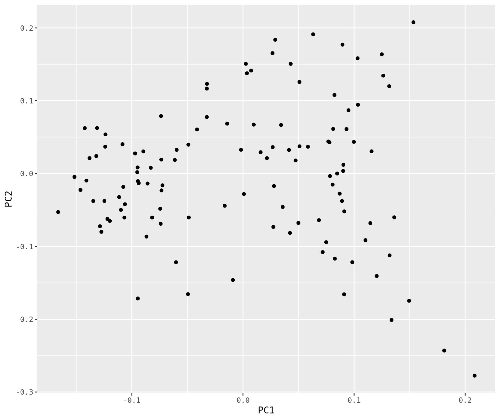
pca_data %>%
ggplot(.,aes(x=PC1, y=PC2)) +
geom_point()
Question
- Based on the sample names, color code the PCA plot by year. Are the two years different in the first two PCs? What about PCs 3 and 4?
We want to use the PCA values as covariates for our GWA. We’re going to use plink for the GWA so we have to follow its format. It wants the first two columns to contain the family ID and sample ID. If you had related individuals, you could use this to show which family each was in, but in our case each individual is a random fish and we don’t expect any to be close relatives. So for each sample we’re using the same value for family ID and sample ID.
pca_data %>%
  select(family.id, sample.id, PC1, PC2, PC3, PC4, PC5) %>%
  write_tsv("Desktop/chinook.gwas.pca.txt")
Upload the chinook.gwas.pca.txt file to your lab_9/info directory on fossa using scp.
The phenotype file I’ve included in the shared directory, so we can copy that over
cp /project/ctb-grego/sharing/lab_9/chinook.date.pheno info/chinook.gwas.pheno.txt
Now we’re ready to run our first GWAS.
plink --vcf vcf/chinook.gwas.vcf.gz \
    --out gwas/chinook.gwas \
    --linear \
    --covar info/chinook.gwas.pca.txt \
    --allow-extra-chr \
    --double-id \
    --pheno info/chinook.gwas.pheno.txt \
    --all-pheno \
    --allow-no-sex
With this command, we’re using a linear model to test the association between this trait and the genotype (since its a quantitative trait). We’re using the first 5 PCs as covariates to control for population stratification. We’re passing the phenotype values in a separate file with the –pheno option.
Now lets plot this in R. Again, use scp to download the chinook.gwas.P1.assoc.linear file. Also download all the files in the sharing/lab_9 directory: “/project/ctb-grego/sharing/lab_9/*”. You will need them for plotting.
gwas <- read_table("Desktop/chinook.gwas.P1.assoc.linear")
head(gwas)
> head(gwas)
# A tibble: 6 × 10
  CHR        SNP      BP A1    TEST  NMISS     BETA    STAT        P X10
  <chr>      <chr> <dbl> <chr> <chr> <dbl>    <dbl>   <dbl>    <dbl> <chr>
1 CM031216.1 .       455 T     ADD      95   -3.09  -1.67   9.79e- 2 NA
2 CM031216.1 .       455 T     COV1     95   40.9    2.86   5.25e- 3 NA
3 CM031216.1 .       455 T     COV2     95 -112     -7.34   9.92e-11 NA
4 CM031216.1 .       455 T     COV3     95   46.6    3.34   1.24e- 3 NA
5 CM031216.1 .       455 T     COV4     95    0.534  0.0378 9.70e- 1 NA
6 CM031216.1 .       455 T     COV5     95   20.8    1.40   1.64e- 1 NA
For each SNP in the genome, we have multiple lines. One of the lines is the association between the SNP and our phenotype (after controlling for covariates), while the others are the effect of the covariate on the SNP. We aren’t particularly interested in the covariate effects, so we can filter those out.
gwas <- gwas %>%
  filter(TEST == "ADD")
Lastly, when plotting GWAS, its easier to visualize -log10(p) values, so lets create that column.
gwas <- gwas %>%
  mutate(log_p = -log10(P))
When making GWA plots, we often have huge numbers of points. If you try to make a figure with millions of points, it often bogs down you computer or results in a pdf file that is way too big to handle. So, an easy work around is to filter points to not plot SNPs that are completely unassociated.
gwas %>%
  filter(log_p > 1) %>%
  ggplot(.,aes(x=BP,y=log_p)) +
  geom_point()
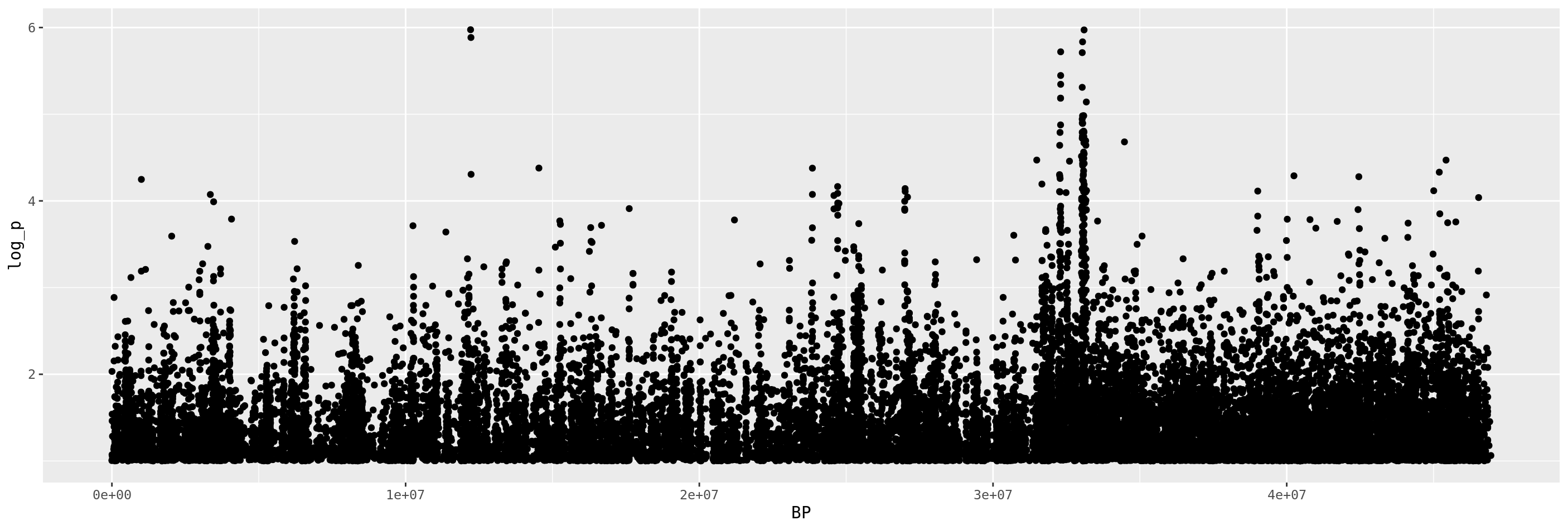
We see a pretty big peak at the right side of the graph, as well as a couple high points midway across the chromosome. Lets zoom in on these.
gwas %>%
  arrange(desc(log_p)) %>%
  head()
# A tibble: 6 × 11
  CHR        SNP         BP A1    TEST  NMISS   BETA  STAT          P X10   log_p
  <chr>      <chr>    <dbl> <chr> <chr> <dbl>  <dbl> <dbl>      <dbl> <chr> <dbl>
1 CM031216.1 .     12211921 C     ADD     114 -12.5  -5.18 0.00000106 NA     5.97
2 CM031216.1 .     33100788 A     ADD     114 -12.2  -5.18 0.00000107 NA     5.97
3 CM031216.1 .     12224440 T     ADD     114 -12.6  -5.13 0.00000130 NA     5.88
4 CM031216.1 .     33049078 T     ADD     114 -12.1  -5.10 0.00000146 NA     5.83
5 CM031216.1 .     32303435 T     ADD     114  -9.04 -5.04 0.00000191 NA     5.72
6 CM031216.1 .     33037939 T     ADD     113 -11.1  -5.04 0.00000195 NA     5.71
top_snps <- gwas %>%
arrange(desc(log_p)) %>%
head(n=10) %>%
pull(BP)
plotting_range <- 200000
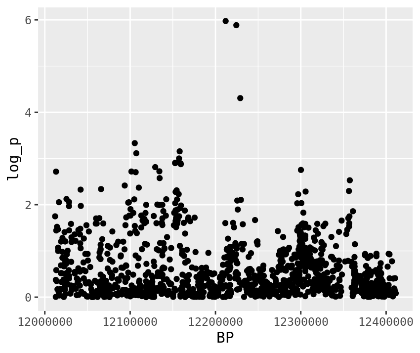
gwas %>%
filter(BP > top_snps[1] - plotting_range,
BP < top_snps[1] + plotting_range) %>%
ggplot(.,aes(x=BP,y=log_p)) +
geom_point()
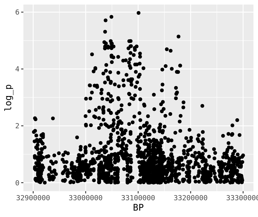
gwas %>%
filter(BP > top_snps[2] - plotting_range,
BP < top_snps[2] + plotting_range) %>%
ggplot(.,aes(x=BP,y=log_p)) +
geom_point()
Now a big question we might as are what genes are under those peaks? We can take a look at that in R. I’ve organized a list of genes, for the chromosome we’re working on.
genes <- read_tsv("Desktop/chinook.genes.txt")
#This filters our SNPs to only those around the highest ranked SNP.
plot_1 <- gwas %>%
  filter(BP > top_snps[1] - plotting_range,
         BP < top_snps[1] + plotting_range) %>%
  ggplot(.,aes(x=BP,y=log_p)) +
  geom_point()
#This adds boxes for genes under the manhattan plot.
#You'll notice I've put a filtering command, within a ggplot command. The filtering command
#makes it so it only plots genes near the outlier SNP.
plot_1 <- plot_1 +
  geom_segment(data = genes %>% filter( start > top_snps[1] - plotting_range,
                                        end < top_snps[1] + plotting_range),
               aes(x = start, y = -0.1, xend = end, yend = -0.1), size = 2, color = "blue")

plot_1
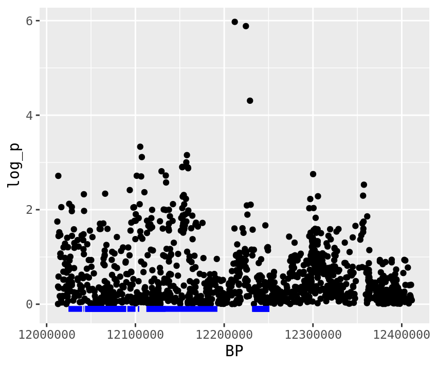
Questions
- What are the gene(s) under the second GWAS peak (around 33 MBp)?
- Choose one of the genes under the peak and BLAST it against the human genome. What is the best hit? HINT: The LOC# is used by NCBI to track genes.
Now that we’ve done some GWAS calculations lets see if we can validate our p-values for one SNP. We’re going to extract the genotypes for one of our top SNPs and run our own linear model.
library(vcfR)
#We have to tell it the path to the original file, not the symbolic link
vcf <- read.vcfR("Desktop/chinook.gwas.vcf.gz")
#extract the genotypes into a tidy table
gt_data <- vcfR2tidy(vcf, format_fields = 'GT' )
gt = gt_data$gt

#This step removes the gt_data, since it hogs memory
rm(gt_data)

#Get the genotypes for your top SNP candidate
top_gt <- gt %>%
  filter(POS == top_snps[1])

phenotypes <- read_tsv("Desktop/chinook.gwas.pheno.txt",
                       col_names = c("Indiv","spacer","phenotype"))

top_gt %>%
  inner_join(phenotypes) %>%
  ggplot(aes(x=gt_GT, y=phenotype)) +
  geom_boxplot()
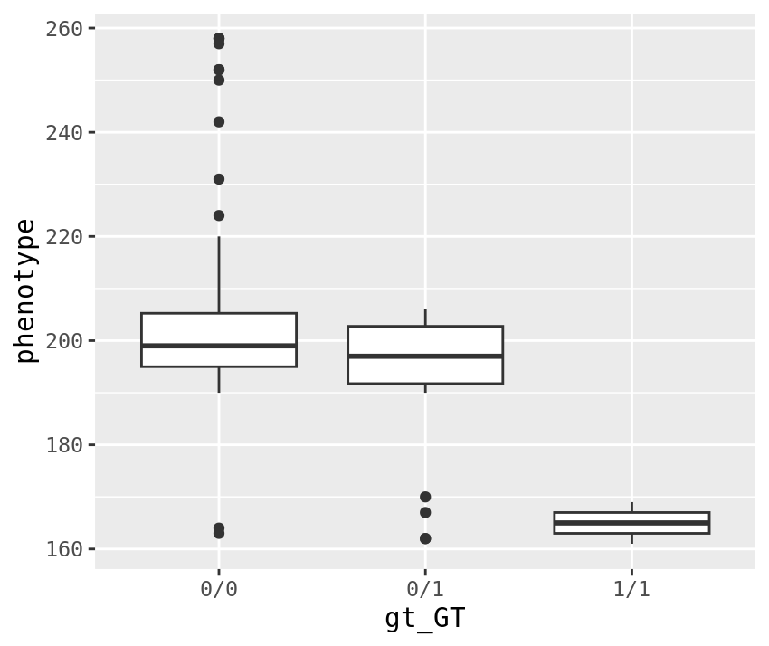
We can see from this that the alternate allele seems to cause a smaller phenotype value. Based on this, we’d probably say that the alternate allele is recessive. Our simple model assumes its additive, but the data fits that model as well which is why the P-value is low. Plink is basically just running a linear model, so lets try that ourselves.
linear_model <- top_gt %>%
  inner_join(phenotypes) %>%
  mutate(genotype_numeric = case_when(gt_GT == "0/0" ~ 0,
                                gt_GT == "0/1" ~ 1,
                                gt_GT == "1/1" ~ 2,
                                TRUE ~ NA)) %>%
  lm(phenotype ~ genotype_numeric, data=.)

summary(linear_model)
Call:
lm(formula = phenotype ~ genotype_numeric, data = .)

Residuals:
    Min      1Q  Median      3Q     Max
-41.965  -8.965  -1.965   5.785  53.035

Coefficients:
                 Estimate Std. Error t value Pr(>|t|)
(Intercept)       204.965      1.828 112.122  < 2e-16 ***
genotype_numeric  -14.001      3.450  -4.058  9.2e-05 ***
---
Signif. codes:  0 ‘***’ 0.001 ‘**’ 0.01 ‘*’ 0.05 ‘.’ 0.1 ‘ ’ 1

Residual standard error: 17.29 on 112 degrees of freedom
Multiple R-squared:  0.1282,	Adjusted R-squared:  0.1204
F-statistic: 16.47 on 1 and 112 DF,  p-value: 9.2e-05
The p-value for this version of the test is 9.2e-5, which is pretty significant. The Estimate is -14, which suggest that each copy of the alternate allele lowers your trait value by 14. One difference is that we didn’t control for the PCAs, so lets try that for our linear model.
pcas <- read_tsv("Desktop/chinook.gwas.pca.txt") %>%
  rename(Indiv = family.id)

linear_model_plus <- top_gt %>%
  inner_join(phenotypes) %>%
  inner_join(pcas) %>%
  mutate(genotype_numeric = case_when(gt_GT == "0/0" ~ 0,
                                      gt_GT == "0/1" ~ 1,
                                      gt_GT == "1/1" ~ 2,
                                      TRUE ~ NA)) %>%
   lm(phenotype ~  PC1 + PC2 + PC3 + PC4 + PC5+ genotype_numeric, data=.)

summary(linear_model_plus)
Call:
lm(formula = phenotype ~ PC1 + PC2 + PC3 + PC4 + PC5 + genotype_numeric,
    data = .)

Residuals:
    Min      1Q  Median      3Q     Max
-38.636  -6.602   1.060   6.247  31.398

Coefficients:
                 Estimate Std. Error t value Pr(>|t|)
(Intercept)       204.620      1.242 164.699  < 2e-16 ***
PC1                49.129     11.647   4.218 5.17e-05 ***
PC2              -113.713     11.666  -9.747  < 2e-16 ***
PC3                57.262     11.710   4.890 3.57e-06 ***
PC4                16.984     11.705   1.451    0.150
PC5               -11.305     12.002  -0.942    0.348
genotype_numeric  -12.542      2.422  -5.178 1.06e-06 ***
---
Signif. codes:  0 ‘***’ 0.001 ‘**’ 0.01 ‘*’ 0.05 ‘.’ 0.1 ‘ ’ 1

Residual standard error: 11.65 on 107 degrees of freedom
Multiple R-squared:  0.6223,	Adjusted R-squared:  0.6011
F-statistic: 29.38 on 6 and 107 DF,  p-value: < 2.2e-16
After controlling for the PCs, the genotype effect is still signficant, suggesting it isn’t only caused by correlation with population stratification. Interestingly, the first three principle components are also correlated with the trait.